Physics AI Explained: How AI Simulates the Real World

Introduction

At the European Centre for Medium-Range Weather Forecasts, every forecast cycle begins the same way. Around 60 million quality-controlled observations from satellites, aircraft, ships and ground stations are combined with a short previous forecast to build a picture of the atmosphere now. That picture is pushed forward by the Integrated Forecasting System, a physics-based model solving the equations of atmospheric motion on a global grid of roughly 9 km spacing [1].

Since February 2025, something else has been running alongside it. ECMWF’s Artificial Intelligence Forecasting System takes the same initial conditions and produces a forecast using a trained neural network rather than a numerical integration of the governing equations, cutting the energy needed per forecast by a factor of about 1,000 [1].

That pairing captures what physics AI actually is. Not a replacement for physics, and not a box that discovers nature on its own, but a second computational instrument running beside the first, with different strengths and different failure modes. This article covers how the main methods work, where they are genuinely used, and what they still cannot do.

What Is Physics AI?

Physics AI is an umbrella term rather than a specific technology. It covers systems built to work with, learn from or approximate physical behaviour, and spans a few families:

• Models that learn from simulation or experimental data while being constrained by known physical laws.
• Models that embed differential equations, conservation laws or symmetries directly into training.
• Surrogate models that approximate the output of an expensive simulation after training on its results.
• Analysis tools that extract structure from large datasets produced by telescopes, colliders or sensor networks.

The colliders behind that data exist to detect the fundamental particles and forces beneath the Standard Model, which is exactly the kind of dataset scientific machine learning is often trained to sift through.

Researchers prefer the term scientific machine learning, which makes the purpose explicit: machine learning aimed at scientific and engineering problems rather than at generating text or images [2].

The distinction from general-purpose generative AI matters more than it might seem. A large language model reproduces statistical patterns in human-written text and is judged on plausibility. A physics-informed model reproduces the behaviour of a physical system, is often penalised during training for violating a governing equation, and is judged on measurable error against known physics.

How Traditional Physics Simulations Work

To see what physics AI adds, it helps to be clear about what it is being compared against.

Most physical systems are described by differential equations: Navier-Stokes for fluids, the heat equation for conduction, Maxwell’s equations for electromagnetism, the Schrödinger equation for non-relativistic quantum systems, or Einstein’s field equations for gravity.

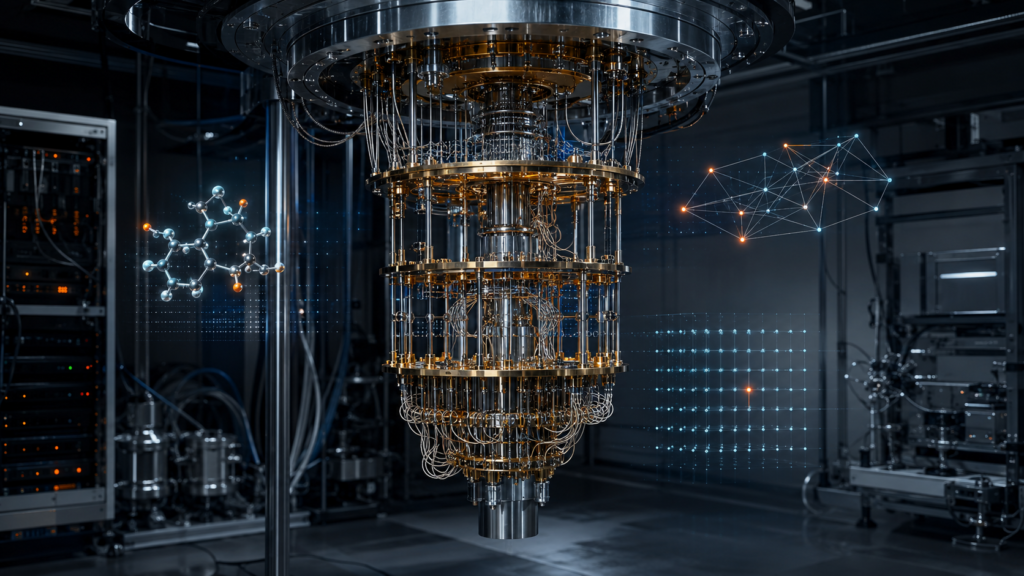
Those last equations are notoriously resistant to a closed-form solution, which is a large part of why general relativity treats gravity as the geometry of spacetime itself rather than a force to be solved for directly. Quantum systems raise a related question from the other direction: quantum computers are being built to simulate quantum systems directly on quantum hardware, rather than solving the Schrödinger equation on a classical machine at all.

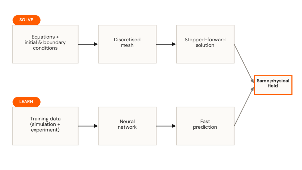
For any realistic geometry or boundary condition, these equations have no closed-form solution, so scientists discretise them. Finite difference, finite volume, finite element and spectral methods all convert a continuous problem into a very large system of algebraic equations a computer can advance step by step, given initial conditions, boundary conditions, a grid, and enough compute to march the solution forward.

The cost comes from resolution. Turbulence, combustion, plasma dynamics and star formation all involve structures spanning many orders of magnitude, and resolving the small ones across a large domain is what drives high-fidelity calculations onto supercomputers. The compensation is that these methods are mathematically understood: accuracy, stability and convergence can be analysed, and conservation of mass, momentum and energy built into the scheme by construction.

How AI Learns Physical Behaviour

Machine learning models begin with data rather than equations. In physics that data comes from three places: high-fidelity simulations produced by conventional solvers, experimental measurements from wind tunnels and instruments, and reanalysis datasets that fuse observations with physical models into a consistent gridded record.

The third category is where a common misunderstanding starts. AI weather models are often described as trained on observations. In practice they are trained on reanalysis, and reanalysis is itself the product of a physics-based model constrained by observations. The learning sits downstream of the physics, not independent of it.

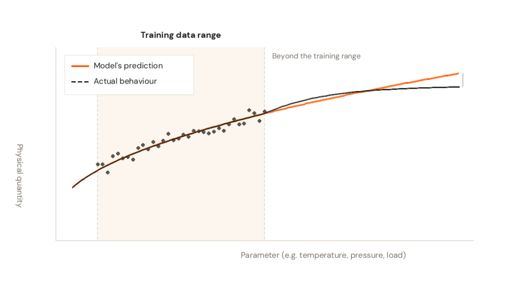
A network is then trained to map inputs, such as an initial state or a set of design parameters, to outputs, such as a future state or a pressure field. What separates this from physics is the gap between correlation and law. A data-driven model can learn that certain inputs tend to be followed by certain outputs without encoding any reason why, and it carries no guarantee of behaving sensibly once conditions move outside what it has seen. Most serious work in physics AI is an attempt to close that gap.

Physics-Informed Neural Networks

Physics-informed neural networks, or PINNs, are the most discussed approach in the field. The modern form was introduced by Raissi, Perdikaris and Karniadakis in 2019 [3].

A neural network is a smooth, differentiable function of its inputs. If those inputs are position and time, the network’s derivatives with respect to them can be computed exactly by automatic differentiation, the same mechanism that produces gradients during training. Those derivatives are substituted directly into the partial differential equation, and the leftover residual measures how badly the current output violates the physics.

That residual becomes part of the loss. The network then minimises two things at once: mismatch with any available data, and violation of the governing equations at sampled points across the domain. Boundary and initial conditions are enforced the same way.

The consequence is that the equations do work data would otherwise have to do. PINNs can be trained on sparse or noisy measurements, and for a forward problem with well-specified boundary conditions, on the equations alone with no observational data. They also suit inverse problems, where an unknown coefficient or source term is inferred from limited measurements, because that unknown can be treated as another trainable parameter.

Where PINNs Struggle

PINNs are not a general replacement for conventional solvers, and the literature is direct about it.

Training is the first problem. The combined loss contains terms of very different scale and character, and their gradients can conflict. Krishnapriyan and colleagues showed that standard PINN formulations fail even on simple convection, reaction and diffusion problems once the coefficients reach moderately difficult regimes, and that the failure lies in the optimisation landscape rather than the network’s capacity [4].

Spectral bias is the second. Networks learn smooth, low-frequency structure far more readily than sharp, high-frequency structure. Wang, Yu and Perdikaris analysed this through neural tangent kernel theory and tied it directly to why PINNs converge unevenly across components of a solution [5]. In practice it shows up as smoothed shocks, blurred boundary layers and missing fine-scale turbulence.

Stiff systems, strongly multiscale problems, sharp gradients and complex geometries all remain difficult, and so does scaling: for large three-dimensional problems, training a PINN to a given accuracy frequently costs more than running a well-implemented finite volume or spectral solver.

Performance is heavily problem-dependent. PINNs are competitive for certain inverse problems, for assimilating scattered measurements, and where a mesh is awkward to build. They are generally not competitive with mature numerical methods on the well-posed forward problems those methods were designed for [2].

Surrogate Models and Neural Operators

The second major strand is faster approximation of expensive simulations. Several distinct things get grouped here, and they are worth separating.

Conventional surrogates and emulators fit a regression model, often polynomial or Gaussian process based, to the outputs of a parameter sweep. Standard engineering practice for decades.

Reduced-order models compress a high-dimensional solution onto a small basis extracted from simulation data, then evolve the system in that compressed space. They keep more physical structure than a black-box fit, but are tied to the regime the basis came from.

Neural operators aim higher. Rather than mapping vectors to vectors, they learn a mapping between function spaces: from an initial-condition or coefficient field to the corresponding solution field. DeepONet builds this from an operator approximation theorem using separate branch and trunk networks [6]. The Fourier Neural Operator parameterises the mapping in the frequency domain, which lets the same trained weights be applied to inputs sampled on different grids [7].

That last property is often called resolution independence, which is too generous. The architecture permits evaluation at a resolution other than the training one. It does not guarantee accuracy survives when that resolution exposes physical scales the training data never contained. Discretisation invariance is a structural property of the model, not a physical guarantee about the answer.

Two further distinctions matter. Training cost is not inference cost: a surrogate answering in milliseconds may have needed thousands of high-fidelity simulations to train, so the speed is amortised and only pays off across many queries. And failure is silent. A conventional solver given an unreasonable problem misbehaves visibly, diverging or failing a conservation check. A surrogate extrapolating beyond its training distribution returns a smooth, plausible, confidently wrong field with nothing flagging the error.

Where Physics AI Is Actually Being Used

Aerospace and Fluid Dynamics

Computational fluid dynamics sits at the centre of aircraft and engine design, and is expensive enough that any credible speedup gets attention.

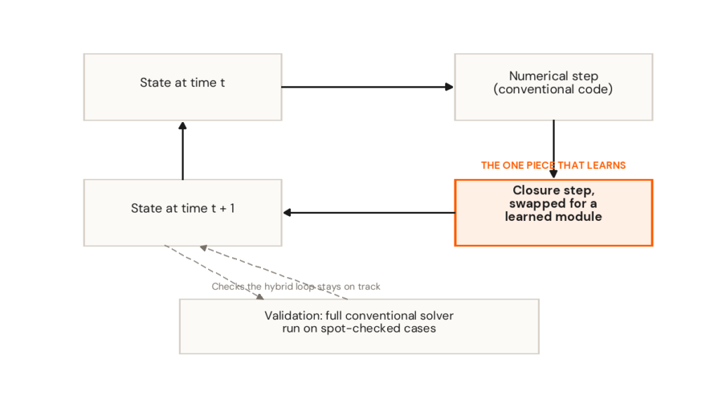
The most promising work does not replace the solver. It replaces a component inside it. Kochkov and colleagues embedded learned interpolation directly into a standard numerical scheme for two-dimensional turbulence, keeping the solver’s structure while letting the network recover accuracy on coarse grids, producing substantial speedups at matched accuracy [8]. Turbulence closure is a second target: the closure term in Reynolds-averaged and large-eddy formulations has always been an approximation, so learning it from high-fidelity data is a natural fit [9].

Claims about industrial aerospace need care. A model trained on one nozzle geometry, one Mach range or one class of aerofoil tells you about that regime, not about a full aircraft with shock interactions, separation and complex geometry. Narrow studies should not be generalised to aerospace simulation as a whole, and for certification-relevant work the binding constraint is verification, validation and uncertainty quantification rather than raw speed.

Weather and Climate

This is where physics AI has moved furthest into operational reality. GraphCast produces ten-day global forecasts of hundreds of variables at 0.25 degree resolution in under a minute, and outperformed the leading operational deterministic system on the large majority of verification targets tested [10]. Pangu-Weather achieved comparable results with a three-dimensional transformer [11], and FourCastNet, still a preprint, showed the same feasibility earlier using Fourier neural operators [12]. ECMWF’s own AIFS became operational in February 2025, with an ensemble version that July [1].

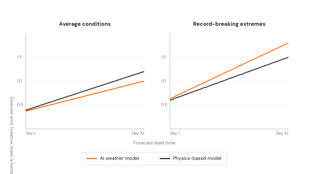
The extremes question is subtler than either enthusiasts or sceptics allow, and the two most careful studies point in different directions. Olivetti and Messori compared IFS HRES against Pangu-Weather and GraphCast and found the data-driven models mostly beat the physics-based model on global error for one to ten day forecasts, and could compete on temperature and wind extremes in most regions [13]. Zhang and colleagues narrowed the question to record-breaking events specifically, and found HRES consistently outperformed GraphCast, Pangu-Weather and FuXi for record heat, cold and wind across nearly all lead times, with the AI models underestimating both the frequency and intensity of records and errors growing with the size of the record [14].

Both can be true, because they measure different things. Average skill and far-tail skill are separate properties, and the tail is exactly where training data is sparsest. For early-warning systems, the tail is the part that matters.

There is also a structural caveat. AIFS runs on initial conditions produced by the same physics-based assimilation system that feeds the IFS [1], so AI forecasting depends on the infrastructure it is described as competing with. Climate modelling is harder still: a weather model needs accuracy for days, while a climate model must stay physically stable and conserve energy across decades of simulated time.

Fusion and Plasma Physics

Tokamak plasmas are nonlinear, turbulent and unforgiving. Control decisions are made on millisecond timescales, and a disruption can damage the machine. Two Nature results anchor what has actually been demonstrated. In 2022, a DeepMind and EPFL collaboration used deep reinforcement learning to control the magnetic coils of the TCV tokamak, training a policy in simulation and transferring it to the physical device to produce and sustain a range of plasma shapes [15]. In 2024, a team on DIII-D trained a controller to steer the plasma away from the conditions that lead to tearing instability, the leading cause of disruptions, rather than reacting after the instability had formed [16].

Both are genuine experimental demonstrations on operating research tokamaks. Neither amounts to autonomous control of a commercial fusion reactor, which does not yet exist. Digital twin work coupling learned surrogates to high-fidelity plasma codes is active, but validated real-time predictive control across all regimes remains open.

Materials Science

Models trained on databases of computed and measured properties can estimate formation energies, band gaps, elastic constants and similar quantities directly from a crystal or molecular structure, letting enormous candidate spaces be filtered before anything is synthesised.

The scale is real. Google DeepMind’s GNoME work reported predictions for over two million structures below the previously known convex hull of stability, around 380,000 of which were released as candidate stable materials [17].

The scrutiny it received is equally instructive. Cheetham and Seshadri examined a randomised subset as experimental materials chemists and reported scant evidence for compounds meeting all three criteria they consider necessary: novelty, credibility and utility. They also noted the predictions cover crystalline inorganic compounds specifically, not materials in the broader sense [18].

The lesson generalises. Computational stability is not synthesisability, synthesisability is not usefulness, and usefulness is not commercial viability. Each gap is crossed in a laboratory, not in a model.

Robotics and Engineering

Here physics AI does unglamorous, useful work. Learned dynamics models give controllers a fast internal prediction of how a system will respond. Structural surrogates predict deflection and stress quickly enough to sit inside a design optimisation loop. State estimators reconstruct quantities that cannot be measured directly. Digital twins couple all of it to a live asset.

The engineering question is always the same: how far can the model be trusted away from the conditions it was fitted to, and what happens when it is wrong.

Astrophysics and Cosmology

Cosmological structure formation is a natural target, because the expensive part, evolving billions of particles under gravity across cosmic time, must be repeated across many parameter sets to compare theory with survey data.

He and colleagues trained a deep network to predict nonlinear structure formation from linear initial conditions, reporting that it outperformed the standard fast analytical approximation [19]. Later work built field-level emulators trained on the Quijote N-body suite, produced specifically to supply training and validation data for machine learning in cosmology [20].

The gravitational collapse these simulations track is also what shapes the invisible scaffolding thought to hold galaxies together, which is why dark matter features so heavily in this kind of simulation.

The dependency is worth stating plainly. These emulators are trained on conventional N-body simulations and validated against them. They accelerate an existing pipeline. They do not remove the need for the simulations that define what correct looks like, or for the survey telescopes generating the observations these simulations are tested against.

Can AI Discover New Laws of Physics?

This question attracts more excitement than the evidence supports, though the underlying research is real. Symbolic regression searches the space of mathematical expressions for a compact formula that fits data. Schmidt and Lipson showed in 2009 that an evolutionary search could recover conservation laws and equations of motion from raw measurements of systems such as double pendulums [21]. Sparse identification of nonlinear dynamics, or SINDy, takes a different route: it builds a library of candidate terms and uses sparse regression to select the few that actually appear in the governing equation, which tends to produce interpretable models from noisy data [22]. AI Feynman exploits structural properties physics equations tend to have, such as symmetry, separability and dimensional consistency, to break a hard symbolic regression problem into easier ones, and recovered a large set of equations from a physics textbook corpus [23].

What these share is that they rediscovered relationships already known to physics, from data generated by systems already understood. That validates the method. It is not the same as discovering a new law.

A physical law clears bars a fitted expression does not. Its terms must correspond to identifiable physical quantities rather than convenient functional forms. It must predict data that played no part in its construction, stay consistent with the rest of physics or show clearly where the existing framework breaks, and survive independent attempts to falsify it.

These tools are strong hypothesis generators, and very good at extracting compact structure where a human might miss it. No AI system has independently established a new fundamental law of nature.

Physics AI Versus Traditional Simulation

The two approaches fail in almost opposite ways, which is the strongest argument for using them together.

Traditional numerical methods are mathematically well characterised. Accuracy, stability and convergence can be analysed, conservation enforced by construction, and they behave sensibly in regimes never previously computed, provided the physics is correctly formulated and adequately resolved. The price is computational cost, and difficulty inferring unknown parameters from sparse measurements.

Physics AI methods are fast at inference, handle high-dimensional inputs, absorb heterogeneous data and suit inverse problems. The price is that error bounds are usually unavailable, conservation is not automatic unless deliberately built in, and reliability degrades unpredictably outside the training distribution. Neither list is a ranking. They describe different tools, which is why most serious work is now hybrid: learned components inside numerical solvers, closure models constrained by physical invariants, surrogates to explore a design space and a conventional solver to verify the final candidates.

The Main Limitations

Four constraints recur across every application above.

Training data defines the domain of validity, and the boundary is rarely marked. The record-breaking weather result is the clearest documented case of what happens beyond it: the models did not visibly break, they systematically underpredicted, and the error grew with the size of the record [14].

Conservation is not free. Unless mass, momentum or energy conservation is enforced through the architecture or the loss, a learned model has no reason to respect it, and small violations compound over long rollouts.

Uncertainty is usually missing or poorly calibrated. Most deployed models return a point estimate, and a prediction without a defensible error bar cannot support a risk decision. Interpretability compounds this: a wrong answer from a numerical solver can usually be traced to a specific term, resolution choice or boundary condition, while a wrong answer from a network is much harder to diagnose.

Verification and validation practice is immature. Engineering has decades of methodology for validating numerical codes against experiment. The equivalent standards for learned models are still being written, and reproducibility across the field is uneven.

None of this makes physics AI unusable. It defines the conditions for using it responsibly.

The Future of Physics AI

The direction of travel is towards systems that are neither purely learned nor purely numerical. Architectures that enforce conservation laws, symmetries and temporal causality by construction rather than by penalty. Hybrid solvers where a learned closure or interpolation sits inside a conventional discretisation, so the numerical scheme still supplies structure and stability. Uncertainty-aware models that report calibrated confidence and detect inputs outside their training distribution. Digital twins that pair fast surrogates with high-fidelity solvers, exploring with one and verifying with the other.

None of this removes the need for the underlying physics. It changes how efficiently the physics can be applied. Physics AI is best understood as a new computational instrument, comparable in kind to the finite element method or the parallel supercomputer, not as a successor to the scientific method.

Conclusion

Physics AI is a family of methods, not a single technology, and it is not replacing physics. It blends governing equations, measured and simulated data, and machine learning to simulate, accelerate or analyse physical systems.

The results are worth taking seriously: operational AI weather forecasting at a fraction of the energy cost, controllers that stabilise real tokamak plasmas, screening pipelines that narrow enormous materials search spaces before anyone touches a furnace, emulators that make cosmological parameter studies affordable.

The limits are equally real. These models fail quietly outside their training data, violate conservation laws unless prevented from doing so, and rarely report how confident they should be. Every application above depends on conventional physics somewhere upstream, in the reanalysis, the N-body suite, or the simulations that produced the training set.

Physics AI works best where it has always worked best: inside the physics, not instead of it.

Frequently Asked Questions

What is physics AI?

Physics AI describes artificial intelligence methods built to model physical systems rather than to generate text or images. It covers physics-informed neural networks, surrogate models, neural operators and reduced-order models, along with tools that analyse large scientific datasets. Researchers more often call the field scientific machine learning. The common thread is that these models are trained against the behaviour of physical systems, and are frequently constrained during training by differential equations, conservation laws or symmetries.

How is physics AI different from generative AI?

They differ in objective, training data and standard of success. A large language model or image generator learns statistical patterns in human-created content, and is judged on whether its output is plausible. A physics AI model learns the behaviour of a physical system from simulation, experiment or reanalysis data, and is judged on measurable error against known physics. Many physics AI models are explicitly penalised during training for violating a governing equation, which has no equivalent in general-purpose generative systems.

Can AI replace traditional physics simulations?

Not in general, and that is not what the current evidence supports. Conventional numerical methods have analysable accuracy and stability, can enforce conservation by construction, and behave predictably in regimes never previously computed. AI models are much faster at inference but usually lack rigorous error bounds and degrade unpredictably outside their training distribution. The productive pattern is hybrid: learned components embedded inside numerical solvers, with conventional solvers retained for verification.

What is a physics-informed neural network?

A physics-informed neural network is trained on two objectives at once. The first is the usual fit to available data. The second is a penalty for violating the governing equations, computed by using automatic differentiation to take derivatives of the network with respect to its space and time inputs, substituting them into the equation, and measuring the leftover residual. This lets the equations substitute for data, so PINNs can work with sparse measurements or, for some forward problems, none at all. They struggle with stiff, multiscale and turbulent problems, and they do not generally outperform mature numerical solvers.

Can AI discover new laws of physics?

Not yet, in any strict sense. Symbolic regression and sparse equation discovery have successfully recovered known conservation laws and equations of motion from experimental and simulated data, which validates the methods. Establishing a new physical law requires more than fitting a compact expression: it needs interpretable terms, predictive success on data not used in its construction, consistency with existing theory, and independent experimental confirmation. AI is currently a strong hypothesis generator, not an autonomous discoverer.

References

1. European Centre for Medium-Range Weather Forecasts. “ECMWF’s AI forecasts become operational.” ECMWF, 25 February 2025. https://www.ecmwf.int/en/about/media-centre/news/2025/ecmwfs-ai-forecasts-become-operational
2. Karniadakis, G. E., Kevrekidis, I. G., Lu, L., Perdikaris, P., Wang, S., and Yang, L. “Physics-informed machine learning.” Nature Reviews Physics, 3(6), 422-440, 2021. https://doi.org/10.1038/s42254-021-00314-5
3. Raissi, M., Perdikaris, P., and Karniadakis, G. E. “Physics-informed neural networks: A deep learning framework for solving forward and inverse problems involving nonlinear partial differential equations.” Journal of Computational Physics, 378, 686-707, 2019. https://doi.org/10.1016/j.jcp.2018.10.045
4. Krishnapriyan, A. S., Gholami, A., Zhe, S., Kirby, R. M., and Mahoney, M. W. “Characterizing possible failure modes in physics-informed neural networks.” Advances in Neural Information Processing Systems, 34, 26548-26560, 2021. https://arxiv.org/abs/2109.01050
5. Wang, S., Yu, X., and Perdikaris, P. “When and why PINNs fail to train: A neural tangent kernel perspective.” Journal of Computational Physics, 449, 110768, 2022. https://doi.org/10.1016/j.jcp.2021.110768
6. Lu, L., Jin, P., Pang, G., Zhang, Z., and Karniadakis, G. E. “Learning nonlinear operators via DeepONet based on the universal approximation theorem of operators.” Nature Machine Intelligence, 3(3), 218-229, 2021. https://doi.org/10.1038/s42256-021-00302-5
7. Li, Z., Kovachki, N., Azizzadenesheli, K., Liu, B., Bhattacharya, K., Stuart, A., and Anandkumar, A. “Fourier neural operator for parametric partial differential equations.” International Conference on Learning Representations, 2021. Preprint: https://arxiv.org/abs/2010.08895
8. Kochkov, D., Smith, J. A., Alieva, A., Wang, Q., Brenner, M. P., and Hoyer, S. “Machine learning-accelerated computational fluid dynamics.” Proceedings of the National Academy of Sciences, 118(21), e2101784118, 2021. https://doi.org/10.1073/pnas.2101784118
9. Vinuesa, R., and Brunton, S. L. “Enhancing computational fluid dynamics with machine learning.” Nature Computational Science, 2(6), 358-366, 2022. https://doi.org/10.1038/s43588-022-00264-7
10. Lam, R., Sanchez-Gonzalez, A., Willson, M., et al. “Learning skillful medium-range global weather forecasting.” Science, 382(6677), 1416-1421, 2023. https://doi.org/10.1126/science.adi2336
11. Bi, K., Xie, L., Zhang, H., Chen, X., Gu, X., and Tian, Q. “Accurate medium-range global weather forecasting with 3D neural networks.” Nature, 619, 533-538, 2023. https://doi.org/10.1038/s41586-023-06185-3
12. Pathak, J., Subramanian, S., Harrington, P., et al. “FourCastNet: A global data-driven high-resolution weather model using adaptive Fourier neural operators.” Preprint, 2022. https://arxiv.org/abs/2202.11214
13. Olivetti, L., and Messori, G. “Do data-driven models beat numerical models in forecasting weather extremes? A comparison of IFS HRES, Pangu-Weather, and GraphCast.” Geoscientific Model Development, 17(21), 7915-7962, 2024. https://doi.org/10.5194/gmd-17-7915-2024
14. Zhang, Z., Fischer, E., Zscheischler, J., and Engelke, S. “Physics-based models outperform AI weather forecasts of record-breaking extremes.” Science Advances, 12(18), eaec1433, 2026. https://doi.org/10.1126/sciadv.aec1433
15. Degrave, J., Felici, F., Buchli, J., et al. “Magnetic control of tokamak plasmas through deep reinforcement learning.” Nature, 602(7897), 414-419, 2022. https://doi.org/10.1038/s41586-021-04301-9
16. Seo, J., Kim, S., Jalalvand, A., Conlin, R., Rothstein, A., Abbate, J., Erickson, K., Wai, J., Shousha, R., and Kolemen, E. “Avoiding fusion plasma tearing instability with deep reinforcement learning.” Nature, 626(8000), 746-751, 2024. https://doi.org/10.1038/s41586-024-07024-9
17. Merchant, A., Batzner, S., Schoenholz, S. S., Aykol, M., Cheon, G., and Cubuk, E. D. “Scaling deep learning for materials discovery.” Nature, 624(7990), 80-85, 2023. https://doi.org/10.1038/s41586-023-06735-9
18. Cheetham, A. K., and Seshadri, R. “Artificial Intelligence Driving Materials Discovery? Perspective on the Article: Scaling Deep Learning for Materials Discovery.” Chemistry of Materials, 36(8), 3490-3495, 2024. https://doi.org/10.1021/acs.chemmater.4c00643
19. He, S., Li, Y., Feng, Y., Ho, S., Ravanbakhsh, S., Chen, W., and Póczos, B. “Learning to predict the cosmological structure formation.” Proceedings of the National Academy of Sciences, 116(28), 13825-13832, 2019. https://doi.org/10.1073/pnas.1821458116
20. Jamieson, D., Li, Y., Alves de Oliveira, R., Villaescusa-Navarro, F., Ho, S., and Spergel, D. N. “Field-level Neural Network Emulator for Cosmological N-body Simulations.” The Astrophysical Journal, 952(2), 145, 2023. https://doi.org/10.3847/1538-4357/acdb6c
21. Schmidt, M., and Lipson, H. “Distilling free-form natural laws from experimental data.” Science, 324(5923), 81-85, 2009. https://doi.org/10.1126/science.1165893
22. Brunton, S. L., Proctor, J. L., and Kutz, J. N. “Discovering governing equations from data by sparse identification of nonlinear dynamical systems.” Proceedings of the National Academy of Sciences, 113(15), 3932-3937, 2016. https://doi.org/10.1073/pnas.1517384113
23. Udrescu, S.-M., and Tegmark, M. “AI Feynman: A physics-inspired method for symbolic regression.” Science Advances, 6(16), eaay2631, 2020. https://doi.org/10.1126/sciadv.aay2631